动手推导Self-attention-译文

清华大学电子信息硕士在读

动手推导Self-attention

在 medium 看到一篇文章从代码的角度,作者直接用 pytorch 可视化了 Attention 的 QKV 矩阵,之前我对 self-Attention 的理解还是比较表面的,大部分时候也是直接就调用 API 来用, 看看原理也挺有意思的,作者同时制作了可在线运行的 colab作为演示,遂翻译给大家一起看看:The illustrations are best viewed on Desktop. A Colab version can be found here, (thanks to Manuel Romero!).

前言:有人问在transformer模型的众多派生BERT，RoBERTa，ALBERT，SpanBERT，DistilBERT，SesameBERT，SemBERT，SciBERT，BioBERT，MobileBERT，TinyBERT和CamemBERT有什么共同点？我们的并不期待你回答都有字母"BERT" .

事实上,答案是 Self-Attention .我们不仅要谈论“BERT”的架构，更正确地说是基于``Transformer架构。基于Transformer的架构主要用于对自然语言理解任务进行建模，避免使用神经网络中的递归神经网络，而是完全依赖Self-Attention`机制来绘制输入和输出之间的全局依存关系。但是，这背后的数学原理是什么？

这就是我们今天要发掘的问题。这篇文章的主要内容是引导您完成Self-Attention模块中涉及的数学运算。在本文结尾处，您应该能够从头开始编写或编写Self-Attention模块。

本文的目的并不是为了通过提供不同的数字表示形式和数学运算来给出Self-attention的直观解释。它也不是为了证明:为什么且如何在Transformers使用中Self-Attention（我相信那里已经有很多东西了）。请注意，本文也没有详细介绍注意力和自我注意力之间的区别。

什么是自注意力机制?

如果你认为自注意力机制类似于注意力机制,那么恭喜你答对了,它们从根本上有很多相同的概念和许多常见的数学运算。

一个self-attention模块输入为 n,输出也为 n.那么在这个模块内部发生了什么?用门外汉的术语来说，self-attention机制允许输入彼此之间进行交互（“self”）并找出它们应该更多关注的区域（“Attention”）。输出是这些交互作用和注意力得分的总和。

实例演示

例子分为以下步骤：

准备输入
初始化权重
导出key, query and value的表示
计算输入1 的注意力得分(attention scores)
计算softmax
将attention scores乘以value
对加权后的value求和以得到输出1
对输入2重复步骤4–7

Note: 实际上，数学运算是向量化的，即所有输入都一起进行数学运算。我们稍后会在“代码”部分中看到此信息。

准备输入

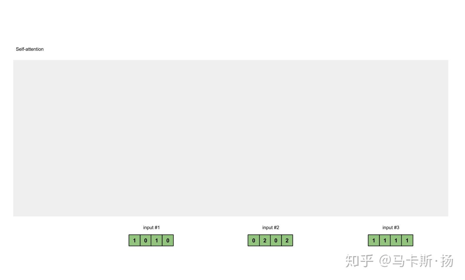
Fig. 1.1: Prepare inputs

在本教程中，我们从3个输入开始，每个输入的尺寸为4。

Input 1: [1, 0, 1, 0] 
Input 2: [0, 2, 0, 2]
Input 3: [1, 1, 1, 1]

初始化权重

每个输入必须具有三个表示形式（请参见下图）。这些表示称为key（橙色），``query（红色）和value`（紫色）。在此示例中，假设我们希望这些表示的尺寸为3。由于每个输入的尺寸均为4，这意味着每组权重的形状都必须为4×3。

Note: 稍后我们将看到value的维度也就是输出的维度。

Fig. 1.2: Deriving key, query and value representations from each input

为了获得这些表示，将每个输入（绿色）乘以一组用于key的权重，另一组用于query的权重和一组value的权重。在我们的示例中，我们如下初始化三组权重。

key的权重

[[0, 0, 1],
[1, 1, 0],
[0, 1, 0],
[1, 1, 0]]

query的权重

[[1, 0, 1],
[1, 0, 0],
[0, 0, 1],
[0, 1, 1]]

value的权重

[[0, 2, 0],
[0, 3, 0],
[1, 0, 3],
[1, 1, 0]]

Note:
在神经网络的设置中，这些权重通常是很小的数，使用适当的随机分布（如高斯，Xavie 和 Kaiming 分布）随机初始化。初始化在训练之前完成一次。*

从每个输入中导出key, query and value的表示

现在我们有了三组值的权重，让我们实际查看每个输入的键，查询和值表示形式。

输入 1 的key的表示形式

               [0, 0, 1]
[1, 0, 1, 0] x [1, 1, 0] = [0, 1, 1]
               [0, 1, 0]
               [1, 1, 0]

使用相同的权重集获得输入 2 的key的表示形式：

               [0, 0, 1]
[0, 2, 0, 2] x [1, 1, 0] = [4, 4, 0]
               [0, 1, 0]
               [1, 1, 0]

使用相同的权重集获得输入 3 的key的表示形式：

               [0, 0, 1]
[1, 1, 1, 1] x [1, 1, 0] = [2, 3, 1]
               [0, 1, 0]
               [1, 1, 0]

一种更快的方法是对上述操作进行矩阵运算：

               [0, 0, 1]
[1, 0, 1, 0]   [1, 1, 0]   [0, 1, 1]
[0, 2, 0, 2] x [0, 1, 0] = [4, 4, 0]
[1, 1, 1, 1]   [1, 1, 0]   [2, 3, 1]

Fig. 1.3a: Derive key representations from each input

让我们做同样的事情以获得每个输入的value表示形式：

               [0, 2, 0]
[1, 0, 1, 0]   [0, 3, 0]   [1, 2, 3] 
[0, 2, 0, 2] x [1, 0, 3] = [2, 8, 0]
[1, 1, 1, 1]   [1, 1, 0]   [2, 6, 3]

Fig. 1.3b: Derive value representations from each input

以及query的表示形式:

               [1, 0, 1]
[1, 0, 1, 0]   [1, 0, 0]   [1, 0, 2]
[0, 2, 0, 2] x [0, 0, 1] = [2, 2, 2]
[1, 1, 1, 1]   [0, 1, 1]   [2, 1, 3]

Fig. 1.3c: Derive query representations from each input

Notes: 实际上，可以将偏差向量 b 添加到矩阵乘法的乘积中。
(译者注:y=w\cdot x+b )

计算输入的注意力得分(attention scores)

为了获得注意力分数，我们首先在输入1的query（红色）与所有key（橙色）（包括其自身）之间取点积。由于有3个key表示（因为我们有3个输入），因此我们获得3个注意力得分（蓝色）。

            [0, 4, 2]
[1, 0, 2] x [1, 4, 3] = [2, 4, 4]
            [1, 0, 1]

Fig. 1.4: Calculating attention scores (blue) from query 1

请注意，在这里我们仅使用输入1的query。稍后，我们将对其他查询重复相同的步骤。

Note: 上面的操作被称为"点积注意力"，是几种sorce之一。其他评分功能包括缩放的点积和拼接。
更多 sorce:https://towardsdatascience.com/attn-illustrated-attention-5ec4ad276ee3

计算softmax

Fig. 1.5: Softmax the attention scores (blue)

将attention scores通过 softmax 函数(蓝色)得到概率

softmax([2, 4, 4]) = [0.0, 0.5, 0.5]

将attention scores乘以value

Fig. 1.6: Derive weighted value representation (yellow) from multiply value (purple) and score (blue)

每个输入的softmax注意力得分（蓝色）乘以其相应的value（紫色）。这将得到3个对齐的向量（黄色）。在本教程中，我们将它们称为"加权值"。

1: 0.0 * [1, 2, 3] = [0.0, 0.0, 0.0]
2: 0.5 * [2, 8, 0] = [1.0, 4.0, 0.0]
3: 0.5 * [2, 6, 3] = [1.0, 3.0, 1.5]

对加权后的value求和以得到输出1

Fig. 1.7: Sum all weighted values (yellow) to get Output 1 (dark green)

对所有加权值(黄色)按元素求和：

  [0.0, 0.0, 0.0]
+ [1.0, 4.0, 0.0]
+ [1.0, 3.0, 1.5]
-----------------
= [2.0, 7.0, 1.5]

得到的向量[2.0, 7.0, 1.5] (深绿)是输出 1 , 它是基于“输入1”的“query表示的形式” 与所有其他key(包括其自身）进行的交互。

对输入2重复步骤4–7

现在我们已经完成了输出1，我们将对输出2和输出3重复步骤4至7。我相信我可以让您自己进行操作。

Fig. 1.8: Repeat previous steps for Input 2 & Input 3

Notes: 因为点积得分函数 query和key的维度必须始终相同.但是value的维数可能与query和key的维数不同。因此输出结果将遵循value的维度。

代码

这里要一份 pytorch 代码 ,pytorch 是一种非常受欢迎的深度学习框架.为了在以下代码段中使用“ @”运算符，.T和None索引的API，请确保您使用的Python≥3.6和PyTorch 1.3.1。只需将它们复制并粘贴到Python / IPython REPL或Jupyter Notebook中即可。

Step 1: 准备输入

import torch

x = [
[1, 0, 1, 0], # Input 1
[0, 2, 0, 2], # Input 2
[1, 1, 1, 1]  # Input 3
]
x = torch.tensor(x, dtype=torch.float32)

Step 2: 初始化权重

w_key = [
[0, 0, 1],
[1, 1, 0],
[0, 1, 0],
[1, 1, 0]
]
w_query = [
[1, 0, 1],
[1, 0, 0],
[0, 0, 1],
[0, 1, 1]
]
w_value = [
[0, 2, 0],
[0, 3, 0],
[1, 0, 3],
[1, 1, 0]
]
w_key = torch.tensor(w_key, dtype=torch.float32)
w_query = torch.tensor(w_query, dtype=torch.float32)
w_value = torch.tensor(w_value, dtype=torch.float32)

Step 3:导出key, query and value的表示

keys = x @ w_key
querys = x @ w_query
values = x @ w_value

print(keys)
# tensor([[0., 1., 1.],
#         [4., 4., 0.],
#         [2., 3., 1.]])

print(querys)
# tensor([[1., 0., 2.],
#         [2., 2., 2.],
#         [2., 1., 3.]])

print(values)
# tensor([[1., 2., 3.],
#         [2., 8., 0.],
#         [2., 6., 3.]])

Step 4: 计算输入的注意力得分(attention scores)

attn_scores = querys @ keys.T

# tensor([[ 2.,  4.,  4.],  # attention scores from Query 1
#         [ 4., 16., 12.],  # attention scores from Query 2
#         [ 4., 12., 10.]]) # attention scores from Query 3

Step 5: 计算softmax

from torch.nn.functional import softmax

attn_scores_softmax = softmax(attn_scores, dim=-1)
# tensor([[6.3379e-02, 4.6831e-01, 4.6831e-01],
#         [6.0337e-06, 9.8201e-01, 1.7986e-02],
#         [2.9539e-04, 8.8054e-01, 1.1917e-01]])

# For readability, approximate the above as follows
attn_scores_softmax = [
[0.0, 0.5, 0.5],
[0.0, 1.0, 0.0],
[0.0, 0.9, 0.1]
]
attn_scores_softmax = torch.tensor(attn_scores_softmax)

Step 6: 将attention scores乘以value

weighted_values = values[:,None] * attn_scores_softmax.T[:,:,None]

# tensor([[[0.0000, 0.0000, 0.0000],
#          [0.0000, 0.0000, 0.0000],
#          [0.0000, 0.0000, 0.0000]],
# 
#         [[1.0000, 4.0000, 0.0000],
#          [2.0000, 8.0000, 0.0000],
#          [1.8000, 7.2000, 0.0000]],
# 
#         [[1.0000, 3.0000, 1.5000],
#          [0.0000, 0.0000, 0.0000],
#          [0.2000, 0.6000, 0.3000]]])

Step 7: 对加权后的value求和以得到输出

outputs = weighted_values.sum(dim=0)

# tensor([[2.0000, 7.0000, 1.5000],  # Output 1
#         [2.0000, 8.0000, 0.0000],  # Output 2
#         [2.0000, 7.8000, 0.3000]]) # Output 3

Note* PyTorch has provided an API for this called* *nn.MultiheadAttention*. However, this API requires that you feed in key, query and value PyTorch tensors. Moreover, the outputs of this module undergo a linear transformation.

Step 8:对输入2重复步骤4–7