AutoEncoder是啥？

不想当算法的风控策略不是好项目经理

本文是https://www.kaggle.com/shivamb/how-autoencoders-work-intro-and-usecases的复现代码，但省去了denoise的部分。一直听encoder decoder但不太理解到底是啥 till i come across this kernal.

目录：

介绍：

1.1 什么是自编码器（AutoEncoders）?

1.2 自编码器（AutoEncoder）是如何工作的？

2. 自编码器的使用场景：

2.1 图像重构（Image Reconstruction）
2.2 seq2seq序列预测（Sequence to Sequence Prediction）

1. 介绍

1.1 什么是自编码器

自编码器是一种特殊的神经网络架构，他的输入和输出是架构是相同的。自编码器是通过无监督的方式来训练来获取输入数据在较低维度的表达。在神经网络的后段这些低纬度的信息表达再被重构回高维的数据表达。一个自编码器可以理解成是一个回归任务，用来预测他的输入（构建一个identity function）。这些神经请网络一般中层都会像下面的图中有一个很瘦的节点，强迫神经网络来构建很高效但又相比浅层更高效的数据表达（again，将前馈中的表达数据压缩以供后续的解码器（Decoder）重构原始的输入。

一个典型的自编码器由三个主要的Components构成：

编码架构（Encoding Architecture）: 编码器架构由一系列逐步递减的的layers构成，并且最后是一个非常低维的表达(Latent View Representation)
潜在的表达？？（Latent View Representation）: 代表可将输入压缩的但是信息得到最大化保存的最低维度
解码架构（Decoding Architecture）：解码架构基本就是编码架构的镜像，只不过每层Layer的神经元个数是逐步递增的。

一个fine tuned的自编码器应该能够完美的重构模型从第一层输入的数据，下面我们将会详细介绍，自编码器的主要应用场景有：

降维
图像压缩
图像降噪
图像生成
特征提取

1.2 自编码器是如何Work的

自编码器的主要原理就是学习高维数据的低维表达，让我们通过一个例子来学习一下这个编码过程。考虑一个表达空间（N维空间），考虑这个N维空间被2个变量表达：x1和x2

from plotly.offline import init_notebook_mode, iplot
import plotly.graph_objs as go
import numpy as np
init_notebook_mode(connected=True)

## 生成随机数据
N = 50
random_x = np.linspace(2, 10, N)
random_y1 = np.linspace(2, 10, N)
random_y2 = np.linspace(2, 10, N)

trace1 = go.Scatter(x = random_x, y = random_y1, mode="markers", name="Actual Data")
trace2 = go.Scatter(x = random_x, y = random_y2, mode="lines", name="Model")
layout = go.Layout(title="2D Data Repersentation Space", xaxis=dict(title="x2", range=(0,12)), 
                   yaxis=dict(title="x1", range=(0,12)), height=400, 
                   annotations= \
                   [dict(x=5, y=5, xref='x', yref='y',  \
                         text='This 1D line is the Data Manifold (where data resides)', \
                showarrow=True,align='center',arrowhead=2,arrowsize=1,arrowwidth=2,
                         arrowcolor='#636363',ax=-120,ay=-30,bordercolor='#c7c7c7',
                borderwidth=2,borderpad=4,bgcolor='orange',opacity=0.8)])

figure = go.Figure(data = [trace1],layout=layout)
iplot(figure)

目前为了表达这些数据我们用了2个维度，X和Y。但实际上我们可以将数据进一步压缩成一维：

线条上的参考点：A
与X轴的夹角L 这样的话，任何一个在线条上点B就可以通过与A轴的距离以及夹角来表达了
用代码表达示例如下：

random_y3 = [2 for i in range(100)]
random_y4 = random_y2 + 1
trace4 = go.Scatter(x = random_x[4:24], y = random_y4[4:300], mode="lines")
trace3 = go.Scatter(x = random_x, y = random_y3, mode="lines")
trace1 = go.Scatter(x = random_x, y = random_y1, mode="markers")
trace2 = go.Scatter(x = random_x, y = random_y2, mode="lines")
layout = go.Layout(xaxis=dict(title="x1", range=(0,12)), yaxis=dict(title="x2", range=(0,12)), height=400,
                   annotations=[dict(x=2, y=2, xref='x', yref='y', text='A', showarrow=True, align='center', arrowhead=2, arrowsize=1, arrowwidth=2, 
                                     arrowcolor='#636363', ax=20, ay=-30, bordercolor='#c7c7c7', borderwidth=2, borderpad=4, bgcolor='orange', opacity=0.8), 
                                dict(x=6, y=6, xref='x', yref='y', text='B', showarrow=True, align='center', arrowhead=2, arrowsize=1, arrowwidth=2, arrowcolor='#636363',
                                     ax=20, ay=-30, bordercolor='#c7c7c7', borderwidth=2, borderpad=4, bgcolor='yellow', opacity=0.8), dict(
                                     x=4, y=5, xref='x', yref='y',text='d', ay=-40), 
                                dict(x=2, y=2, xref='x', yref='y', text='angle L', ax=80, ay=-10)], title="2D Data Repersentation Space", showlegend=False)
data = [trace1, trace2, trace3, trace4]
figure = go.Figure(data = data, layout = layout)
iplot(figure)



#################

random_y3 = [2 for i in range(100)]
random_y4 = random_y2 + 1
trace4 = go.Scatter(x = random_x[4:24], y = random_y4[4:300], mode="lines")
trace3 = go.Scatter(x = random_x, y = random_y3, mode="lines")
trace1 = go.Scatter(x = random_x, y = random_y1, mode="markers")
trace2 = go.Scatter(x = random_x, y = random_y2, mode="lines")
layout = go.Layout(xaxis=dict(title="u1", range=(1.5,12)), yaxis=dict(title="u2", range=(1.5,12)), height=400,
                   annotations=[dict(x=2, y=2, xref='x', yref='y', text='A', showarrow=True, align='center', arrowhead=2, arrowsize=1, arrowwidth=2, 
                                     arrowcolor='#636363', ax=20, ay=-30, bordercolor='#c7c7c7', borderwidth=2, borderpad=4, bgcolor='orange', opacity=0.8), 
                                dict(x=6, y=6, xref='x', yref='y', text='B', showarrow=True, align='center', arrowhead=2, arrowsize=1, arrowwidth=2, arrowcolor='#636363',
                                     ax=20, ay=-30, bordercolor='#c7c7c7', borderwidth=2, borderpad=4, bgcolor='yellow', opacity=0.8), dict(
                                     x=4, y=5, xref='x', yref='y',text='d', ay=-40), 
                                dict(x=2, y=2, xref='x', yref='y', text='angle L', ax=80, ay=-10)], title="Latent Distance View Space", showlegend=False)
data = [trace1, trace2, trace3, trace4]
figure = go.Figure(data = data, layout = layout)
iplot(figure)

但目前的核心问题其实是用什么样的逻辑我们才可以使得点B能够通过点A以及夹角L来表达，在B，A，L应该找一个什么样的公式表达。这个问题的答案非常直接：没有一个定死的方程，但是我们可以通过无监督的学习过程来得到一个潜在的解。用简单的话来说：学习的过程可以类比成把B 变成A和L的参数组合的过程。接下来让我们从编码器的角度来理解一下这个过程。

考虑一个没有隐藏层的自编码器，x1和x2被编码成更低维的表达，然后在后续处理中被project回x1和x2两个点（示意图如下）

第一步：在低维找到数据点的表达

如果数据点分别是A和B，那么我们的表达空间就是：点A(X1A,X2A)
点B(X1B,X2B)
这样的话他们在低维上的表达就是：
(X1A,X2A)-->(0,0)
(X2B,X2B)-->(u1B,u2B)

点A：(0,0)
点B：(u1B,u2B)

u1b和u2b分别可以被原始坐标系中的两点距离表达.
u1b = x1b-x1a
u2b = x2b-x2a

第二步：用距离d和角度l来表达点

现在u1b和u2b可以分别用距离d和角度l来表达，如果我们把数据朝着水平轴转l度，那么l就会变成0 ，也就是说：
=>转换前：(d, L)
=>转换后：(d, 0) (旋转后)
这就是在编码阶段的输出，用神经网络中权重w和偏置b来表达就是：
=> (d,0)=W(u1B,u2B)
=> (encoding)
W就是隐藏的权重矩阵，既然我们知道解码过程就是编码过程的倒置，所以解码过程就可以写成
=> (u1B,u2B) = Inverse(W).(d, 0)
=> (decoding)

到这一步，我们就可以确认我们的数据点(x1，x2)在低维空间的表达就是(d,0)。相似的，在解码层面解码的过程中，我们将把数据还原成(x1,x2)。不过需要注意的事，在不同类型的数据中，我们的编码解码等式是不一样的，我们接下来用一个二维的数据来进行举例：

不同的数据不同的规则

在刚刚的例子中，我们把线性的数据投在了一维数据上，并用角度L来表达，但如果数据不能被这么处理呢？考虑下面这个例子

import matplotlib.pyplot as plt 
import numpy as np
fs = 100 # sample rate 
f = 2 # the frequency of the signal
x = np.arange(fs) # the points on the x axis for plotting
y = [ np.sin(2*np.pi*f * (i/fs)) for i in x]

%matplotlib inline
plt.figure(figsize=(15,4))
plt.stem(x,y, 'r', );
plt.plot(x,y);

在这种数据集中，我们主要的问题就是要得到原始数据但一维上的表达，但同时不能失去任何信息。但像上图这种情况我们根本不可能像之前那样通过挪转腾挪来得到数据的无损表达。

那么神经网络是怎么解决这个问题的呢？在高维空间上，神经网络可以通过扭曲我们的空间来得到数据的线性表达。我们的自编码器就是通过这个能力来学习到高维数据的低维空间表达的（下图是一个例子）

2. 构建及使用场景

2.1 使用场景1：图像重构
直接开始写代码

from keras.layers import Dense, Input, Conv2D,LSTM,MaxPool2D,UpSampling2D
from sklearn.model_selection import train_test_split
from keras.callbacks import EarlyStopping
from keras.utils import to_categorical
from numpy import argmax, array_equal
import matplotlib.pyplot as plt
from keras.models import Model
# from imgaug import augmenters
from random import randint
import pandas as pd
import numpy as np

### read dataset 
train = pd.read_csv("fashion-mnist_train.csv")
train_x = train[list(train.columns)[1:]].values
train_y = train['label'].values

## normalize and reshape the predictors  
train_x = train_x / 255

## create train and validation datasets
train_x, val_x, train_y, val_y = train_test_split(train_x, train_y, test_size=0.2)

## reshape the inputs
train_x = train_x.reshape(-1, 784)
val_x = val_x.reshape(-1, 784)

数据准备完成后开始构建网络

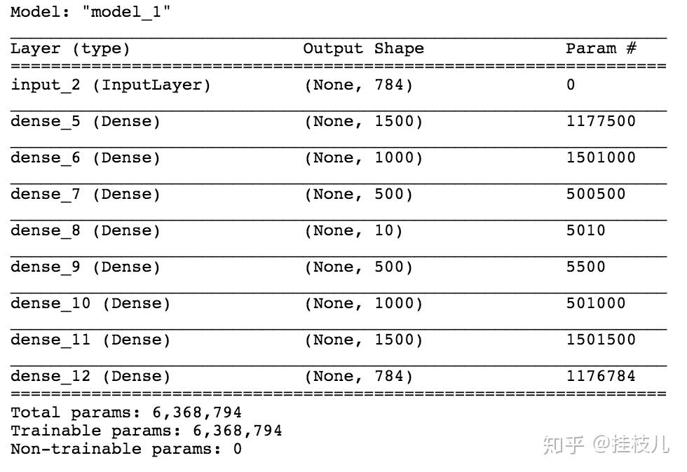
我们够见一个分别由2000个，1200个，500个神经元构成的编码器架构。我们的编码架构将会与一个10个神经元的中间层链接，然后再一次被后续的解码结构500，1200，2000个神经元去解码。最后一层的神经元数与输入层的神经元数相同，代码定义如下：

input_layer = Input(shape=(784,))

# 编码层
encode_layer1 = Dense(1500,activation='relu')(input_layer)
encode_layer2 = Dense(1000,activation='relu')(encode_layer1)
encode_layer3 = Dense(500,activation='relu')(encode_layer2)

# 低维表达层面
latent_view   = Dense(10, activation='sigmoid')(encode_layer3)

# 解码层

decode_layer1 = Dense(500,activation='relu')(latent_view)
decode_layer2 = Dense(1000,activation='relu')(decode_layer1)
decode_layer3 = Dense(1500,activation='relu')(decode_layer2)

# 输出层
output_layer = Dense(784)(decode_layer3)

model = Model(input_layer,output_layer)
# 来看看模型的summary
model.summary()

接下来进行模型的训练

这里需要注意我们的样本的特征和标签都是train_x

model.compile(optimizer='adam',loss='mse')
early_stopping =  \
EarlyStopping(monitor = 'val_loss',min_delta=0,patience=10,verbose=1,mode='auto')
model.fit(train_x,train_x,epochs=20,batch_size=2048,validation_data=(val_x,val_x), 
          callbacks=[early_stopping])

然后我们来对数据做一个预测，然后把图画出来

标签原图：

preds = model.predict(val_x)
from PIL import Image
%matplotlib inline
f,ax = plt.subplots(1,5)
f.set_size_inches(80,40)



for i in range(5):
    ax[i].imshow(val_x[i].reshape(28,28))
plt.show()

然后画一下我们经过编码解码后的图像

f, ax = plt.subplots(1,5)
f.set_size_inches(80, 40)
for i in range(5):
    ax[i].imshow(preds[i].reshape(28, 28))
plt.show()

2.2 序列预测（Sequence to Sequence Prediction using AutoEncoders）

刚刚的例子是二维的数据，序列预测我们面对的肯定就是一维数据，比较典型的就是时序问题或者文本问题，这类模型我们一般都会使用LSTM来进行处理.这个kernal这块有很多是借鉴这篇文章的。

自编码器的架构 这个use case下的架构道理和之前那个其实一样，会有一个编码器来对输入序列进行编码，一个解码器来对编码后的数据进行解码。序列模型一般使用LSTM，先简单介绍下什么是LSTM：：
LSTM也叫长短记忆（Long Short-Term Memory）,这类神经网络一层内有很多hidden state，同时LSTM又带入了gate的概念能够保证网络在前馈过程中携带足够的信息，这个功能使得LSTM在实际性能上比RNN要出众很多。
我们可以通过定义LSTM的记忆unit个数，每个unit都有一个内部的状态，一般用c来表示，然后输出一个隐层的装填，用h来表示.

道理讲完现在开码，我们的代码由2个部分构成：

一个编码器，接受一个序列数据，返回目前LSTM的状态.
一个解码器，接受一个序列数据以及LSTM的状态，返回输出序列。
我们将存储LSTM的隐层装填，这样的话就可以在预测未知的数据时复用数据。

首先，我们定义一个用来生成一个序列数据（包含相同长度的不同信息）的函数：

X1代表输入的序列包含随机数据
X2代表填充后的序列
y代表目标序列

def dataset_preparation(n_in,n_out,n_unique,n_samples):
    x1,x2,y = [],[],[]
    
    for _ in range(n_samples):
        inp_seq = [randint(1,n_unique-1) for _ in range(n_in)]
        
        #目标序列
        target = inp_seq[:n_out]
        
        # padding
        target_seq = list(reversed(target))
        seed_seq = [0] + target_seq[:-1]
        
        # 将数据转变成Keras的格式
        
        x1.append(to_categorical([inp_seq],num_classes=n_unique))
        x2.append(to_categorical([seed_seq],num_classes=n_unique))
        y.append(to_categorical([target_seq],num_classes=n_unique))
        
    # 去除多余的axis
    x1 = np.squeeze(np.array(x1),axis=1)
    x2 = np.squeeze(np.array(x2),axis=1)
    y = np.squeeze(np.array(y),axis=1)
    return x1,x2,y


samples = 100000
features = 51
inp_size = 6
out_size = 3

inputs, seeds, outputs = dataset_preparation(inp_size,out_size,features,samples)
print("Shapes: ", inputs.shape, seeds.shape, outputs.shape)
print ("Here is first categorically encoded input sequence looks like: ", )
inputs[0][0]

>>>> Shapes:  (100000, 6, 51) (100000, 3, 51) (100000, 3, 51)
Here is first categorically encoded input sequence looks like: 
array([0., 0., 0., 0., 0., 0., 0., 0., 0., 0., 0., 0., 0., 0., 0., 0., 0.,
       0., 0., 0., 0., 0., 0., 0., 0., 0., 1., 0., 0., 0., 0., 0., 0., 0.,
       0., 0., 0., 0., 0., 0., 0., 0., 0., 0., 0., 0., 0., 0., 0., 0., 0.],
      dtype=float32)

接下来定义模型架构

def define_models(n_input,n_output):
    
    # 定义编码架构,输入是序列，输出是编码状态
    
    encoder_inputs = Input(shape=(None, n_input))
    encoder = LSTM(128, return_state=True)
    encoder_outputs, state_h, state_c = encoder(encoder_inputs)
    encoder_states = [state_h, state_c]
    
    
    # 定义编码到解码结构，输入是一个种子序列，输出是解码状态，解码输出
    
    decoder_inputs = Input(shape=(None, n_output))
    decoder_lstm = LSTM(128, return_sequences=True, return_state=True)
    decoder_outputs, _, _ = decoder_lstm(decoder_inputs, initial_state=encoder_states)
    decoder_dense = Dense(n_output, activation='softmax')
    decoder_outputs = decoder_dense(decoder_outputs)
    model = Model([encoder_inputs, decoder_inputs], decoder_outputs)
    
    
    # 定义解码架构，输入是目前状态，编码序列，输出是解码序列
    
    encoder_model = Model(encoder_inputs, encoder_states)
    decoder_state_input_h = Input(shape=(128,))
    decoder_state_input_c = Input(shape=(128,))
    decoder_states_inputs = [decoder_state_input_h, decoder_state_input_c]
    decoder_outputs, state_h, state_c = decoder_lstm(decoder_inputs, initial_state=decoder_states_inputs)
    decoder_states = [state_h, state_c]
    decoder_outputs = decoder_dense(decoder_outputs)
    decoder_model = Model([decoder_inputs] + decoder_states_inputs, [decoder_outputs] + decoder_states)

    return model, encoder_model, decoder_model

autoencoder, encoder_model, decoder_model = define_models(features, features)

看看模型架构

autoencoder.compile(optimizer='adam', loss='categorical_crossentropy', metrics=['acc'])
autoencoder.fit([inputs, seeds], outputs, epochs=1)


def reverse_onehot(encoded_seq):
    return [argmax(vector) for vector in encoded_seq]

def predict_sequence(encoder, decoder, sequence):
    output = []
    target_seq = np.array([0.0 for _ in range(features)])
    target_seq = target_seq.reshape(1, 1, features)

    current_state = encoder.predict(sequence)
    for t in range(out_size):
        pred, h, c = decoder.predict([target_seq] + current_state)
        output.append(pred[0, 0, :])
        current_state = [h, c]
        target_seq = pred
    return np.array(output)

for k in range(5):
    X1, X2, y = dataset_preparation(inp_size, out_size, features, 1)
    target = predict_sequence(encoder_model, decoder_model, X1)
    print('\nInput Sequence=%s SeedSequence=%s, PredictedSequence=%s' 
          % (reverse_onehot(X1[0]), reverse_onehot(y[0]), reverse_onehot(target)))

这个Kernal还参考了其他文章，lstm的部分我自己也还没太看明白，继续肝！

发布于 2020-04-03 08:13

Keras

seq2seq